Running the MLOps Fraud Detection Demo

The following steps describes how you can use this pattern in a demo.

Get the MLFlow Route using command-line

You can use the OC command to get the hostname through:

oc get svc mlflow-server -n mlops -o go-template --template='{{.metadata.name}}.{{.metadata.namespace}}.svc.cluster.local{{println}}'

The port you will find with:

oc get svc mlflow-server -n mlops -o yaml

apiVersion: v1
kind: Service
metadata:
...
spec:
  clusterIP: 172.31.112.122
  clusterIPs:
  - 172.31.112.122
  internalTrafficPolicy: Cluster
  ipFamilies:
  - IPv4
  ipFamilyPolicy: SingleStack
  ports:
  - name: mlflow-server
    port: 8080
    protocol: TCP
    targetPort: mlflow-server
  - name: oauth
    port: 8443
    protocol: TCP
    targetPort: oauth-proxy
  selector:
    app.kubernetes.io/instance: mlflow-server
    app.kubernetes.io/name: mlflow-server
  sessionAffinity: None
  type: ClusterIP
status:
  loadBalancer: {}

It is the port for spec.ports.name mlflow-server. In this case the server:port is: mlflow-server.mlops.svc.cluster.local:8080. Use this value when creating the work bench:

MLFLOW_ROUTE=http://mlflow-server.mlops.svc.cluster.local:8080

Create a OpenShift Data Science workbench

Start by opening up OpenShift Data Science by clicking image::../images/grid.png in the top right and choosing "Red Hat OpenShift Data Science".

Under Data Science Projects, create a new project by selecting "Create data science project". This is where you will build and train the model. This will also create a namespace in OpenShift which is where the application will be running after the model training is done. In the example the project is called 'Credit Card Fraud'.

You may change the project name to something different but be aware that steps further down in the demo may also need to change.

After the project has been created, create a workbench where we can run Jupyter. There are a few important settings here that we need to set:

Name: Credit Fraud Model
Notebook Image: Standard Data Science
Deployment Size: Small
Environment Variable: Add a new one that’s a Config Map → Key/value and enter
- Get value by running the following form the commandline:
  oc get service mlflow-server -n mlops -o go-template --template='http://{{.metadata.name}}.{{.metadata.namespace}}.svc.cluster.local:8080{{println}}'
- Key: MLFLOW_ROUTE
- Value: http://<route-to-mlflow>:8080, replacing <route-to-mlflow> and 8080 with the route and port respectfully, that we found in step one. In this case it is http://mlflow-server.mlflow.svc.cluster.local:8080
Cluster Storage: Create new persistent storage - Call it "Credit Fraud Storage" and set the size to 20GB.

Open the workbench and login if needed.

Train the model

When inside the workbench (Jupyter), we are going to clone a GitHub repository which contains everything we need to train (and run) our model. You can clone the GitHub repository by pressing the GitHub button in the left side menu (see image), then select "Clone a Repository" and enter this GitHub URL:+

https://github.com/validatedpatterns/mlops-fraud-detection/tree/main/demo/credit-fraud-detection-demo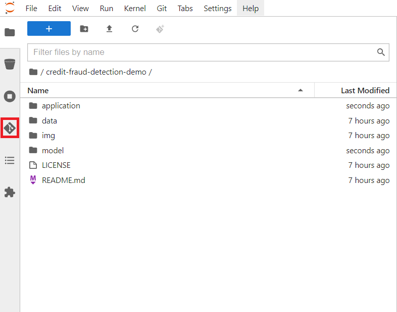

Figure 1. Open the model folder

Open up the folder that was added (credit-fraud-detection-demo). It contains:

Data for training and evaluating the model.
A notebook (model.ipynb) inside the model folder with a Deep Neural Network model we will train.
An application (model_application.py) inside the application folder that fetchs the trained model from MLFlow and runs a prediction on it whenever it receives user input.

The model.ipynb is used to build and train the model. Open that file and take a look inside. There is documentation outlining what each cell does. Of particular interest for this demo are the last two cells.The second to last cell contains the code for setting up MLFlow tracking:

mlflow.set_tracking_uri(MLFLOW_ROUTE)
mlflow.set_experiment("DNN-credit-card-fraud")
mlflow.tensorflow.autolog(registered_model_name="DNN-credit-card-fraud")

mlflow.set_tracking_uri(MLFLOW_ROUTE) points to where to should the MLFlow data. mlflow.set_experiment("DNN-credit-card-fraud") tells MLFlow to create an experiment with a name string. In this case it is called "DNN-credit-card-fraud" because it’s a Deep Neural Network. mlflow.tensorflow.autolog(registered_model_name="DNN-credit-card-fraud") enables autologging of several variables (such as accuracy, loss, etc) - so there is no need to manually track those variables. It also automatically uploads the model to MLFlow after training completes. Here the model is named the same as the experiment.

The last cell contains the training code:

with mlflow.start_run():
    epochs = 2
    history = model.fit(X_train, y_train, epochs=epochs, \
                        validation_data=(scaler.transform(X_val),y_val), \
                        verbose = True, class_weight = class_weights)

    y_pred_temp = model.predict(scaler.transform(X_test))

    threshold = 0.995

    y_pred = np.where(y_pred_temp > threshold, 1,0)
    c_matrix = confusion_matrix(y_test,y_pred)
    ax = sns.heatmap(c_matrix, annot=True, cbar=False, cmap='Blues')
    ax.set_xlabel("Prediction")
    ax.set_ylabel("Actual")
    ax.set_title('Confusion Matrix')
    plt.show()

    t_n, f_p, f_n, t_p = c_matrix.ravel()
    mlflow.log_metric("tn", t_n)
    mlflow.log_metric("fp", f_p)
    mlflow.log_metric("fn", f_n)
    mlflow.log_metric("tp", t_p)

    model_proto,_ = tf2onnx.convert.from_keras(model)
    mlflow.onnx.log_model(model_proto, "models")

with mlflow.start_run(): is used to tell MLFlow to start a run, and it contains our training code to define exactly what code belongs to the "run". Most of the rest of the code in this cell is normal model training and evaluation code, but at the bottom ar calls to send specific custom metrics to MLFlow through mlflow.log_metric() and then convert the model to ONNX. This is because ONNX is one of the standard formats for Red Hat OpenShift AI Model Serving which will be used later.

Next run all the cells in the notebook from top to bottom, either by clicking Shift-Enter on every cell, or by going to Run→Run All Cells in the very top menu. If everything is set up correctly it will train the model and push both the run and the model to MLFlow. The run is a record with metrics of how the run went, while the model is the actual tensorflow and ONNX model which will be used later for inference. There may be some warning messages in the last cell related to MLFlow, as long as the final progress bar appears for the model being pushed to MLFlow all is fine:

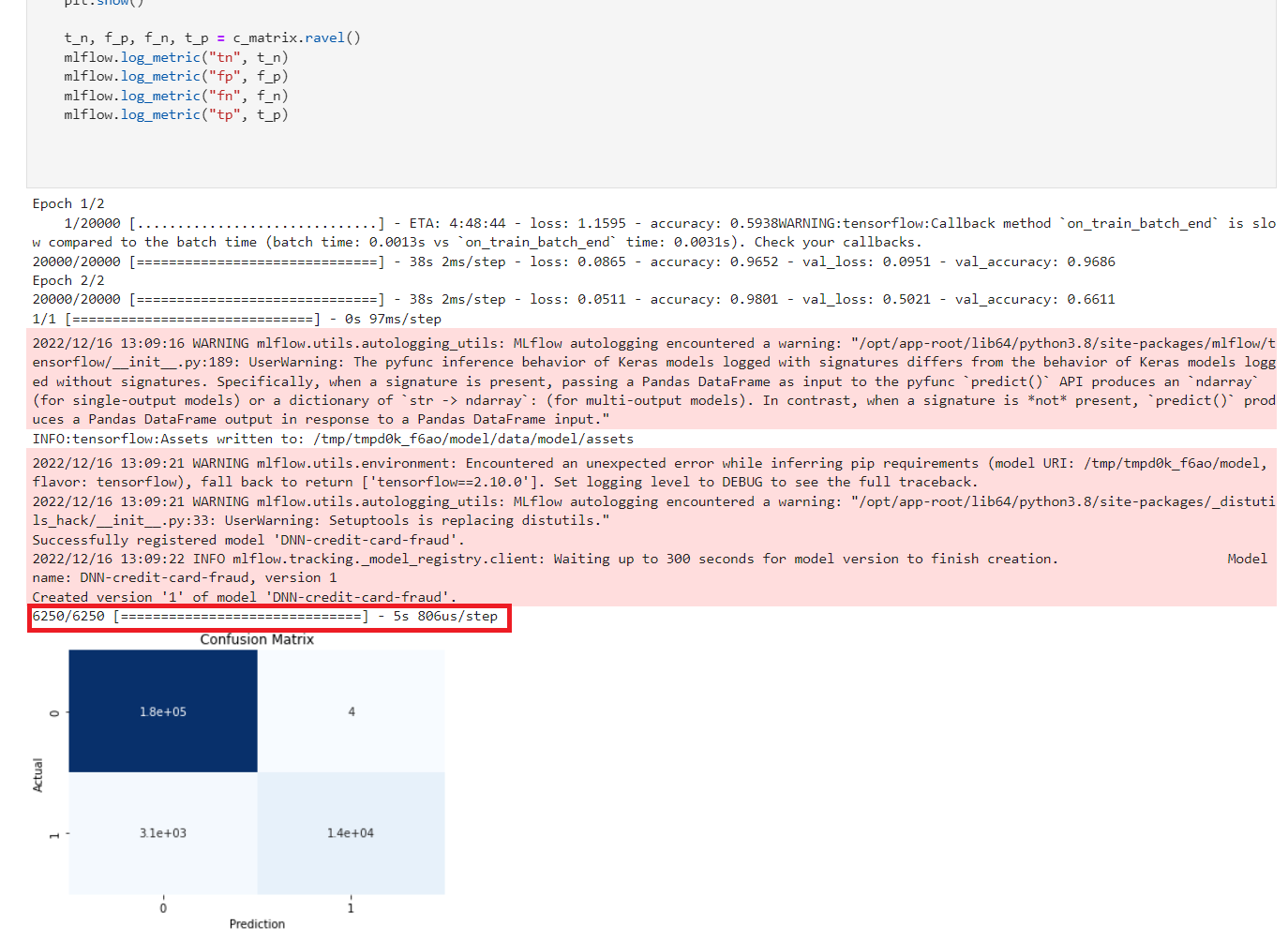
Figure 2. The trained model

View the model in MLFlow

Take a look at how the model looks inside MLFlow now that it has been trained. Open the MLFlow UI from the shortcut.

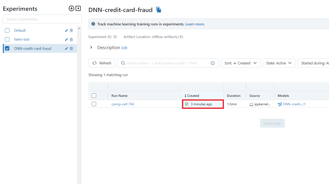
Figure 3. View the trained model in MLFlow

The Full Path of the model is required in the next section in order to serve the model. So keep the MLflow DNN-credit-card-fraud dialog open.

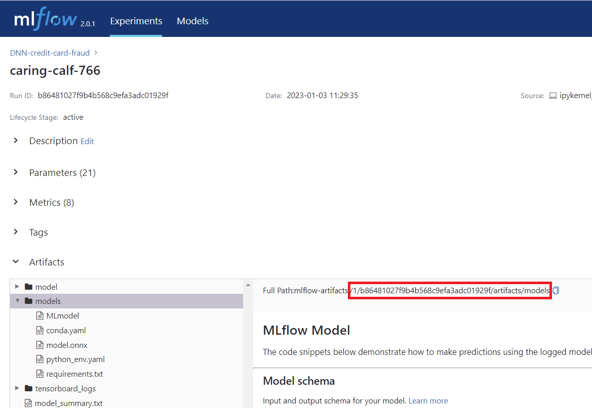
Figure 4. MLFlow Model Path

Serve the model

The model can be served using Red Hat OpenShift AI Model Serving or by using the model directly from MLFlow. This section shows how you serve it with Red Hat OpenShift AI Model Serving, as it scales better for large applications and load. The bottom of this section goes through how to use MLFlow instead.

To start, go to your Red Hat OpenShift AI Project and click "Add data connection". This data connection connects to storage from where the model can be loaded.

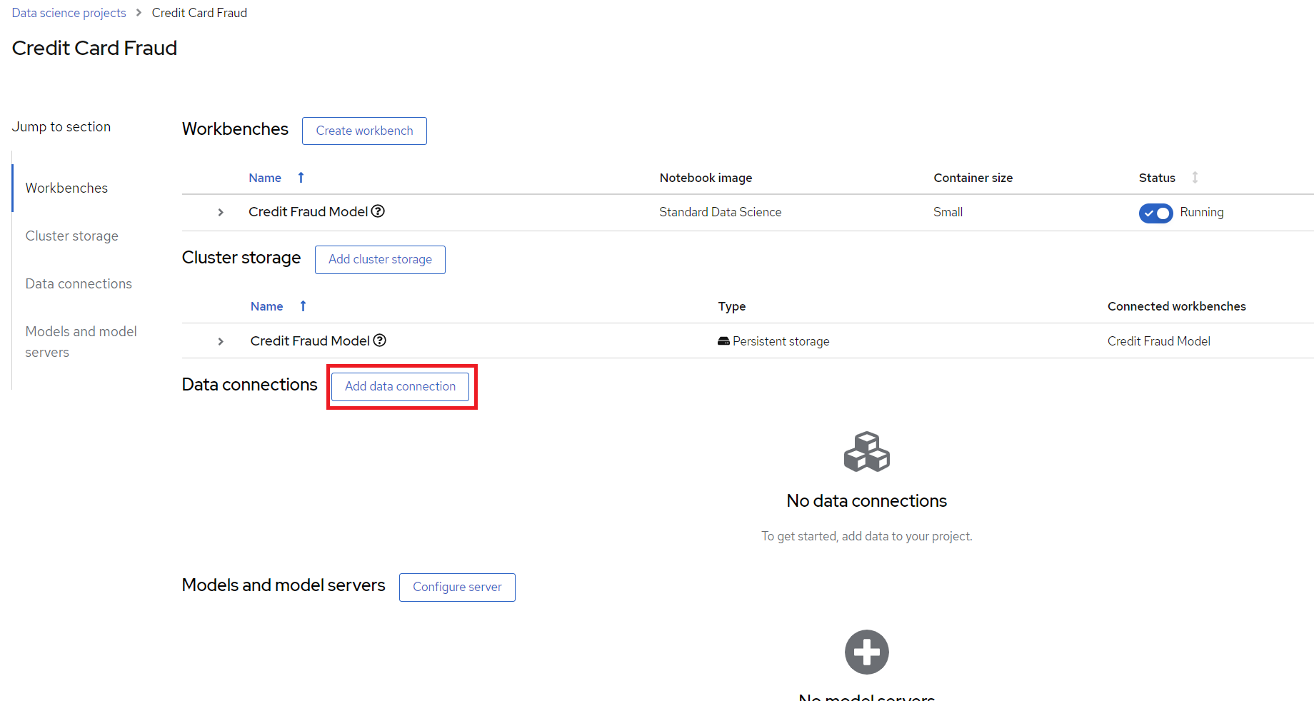
Figure 5. Add data connection

Some details need to be added for the data connection. Assuming that you set up MLFlow according to this guide and have it connected to Red Hat Open Data Foundation. If that’s not the case then enter the relevant details for your usecase. Copy the code section below and run it all to find your values.

echo "==========Data connections Start==========="
echo "Name \nmlflow-connection"
echo
echo AWS_ACCESS_KEY_ID
oc get secrets mlflow-server -n mlops -o json | jq -r '.data.AWS_ACCESS_KEY_ID|@base64d'
echo
echo AWS_SECRET_ACCESS_KEY
oc get secrets mlflow-server -n mlops -o json | jq -r '.data.AWS_SECRET_ACCESS_KEY|@base64d'
echo
echo AWS_S3_ENDPOINT
oc get configmap mlflow-server -n mlops -o go-template --template='http://{{.data.BUCKET_HOST}}{{println}}'
echo
echo "AWS_DEFAULT_REGION \nus-east-2"
echo
echo AWS_S3_BUCKET
oc get configmap mlflow-server -n mlops -o go-template --template='{{.data.BUCKET_NAME}}{{println}}'
echo
echo "Connected workbench \nCredit Fraud Model"
echo "==========Data connections End==========="

After pressing the "Add data connection" button. Here is an example of how to fill the form out:

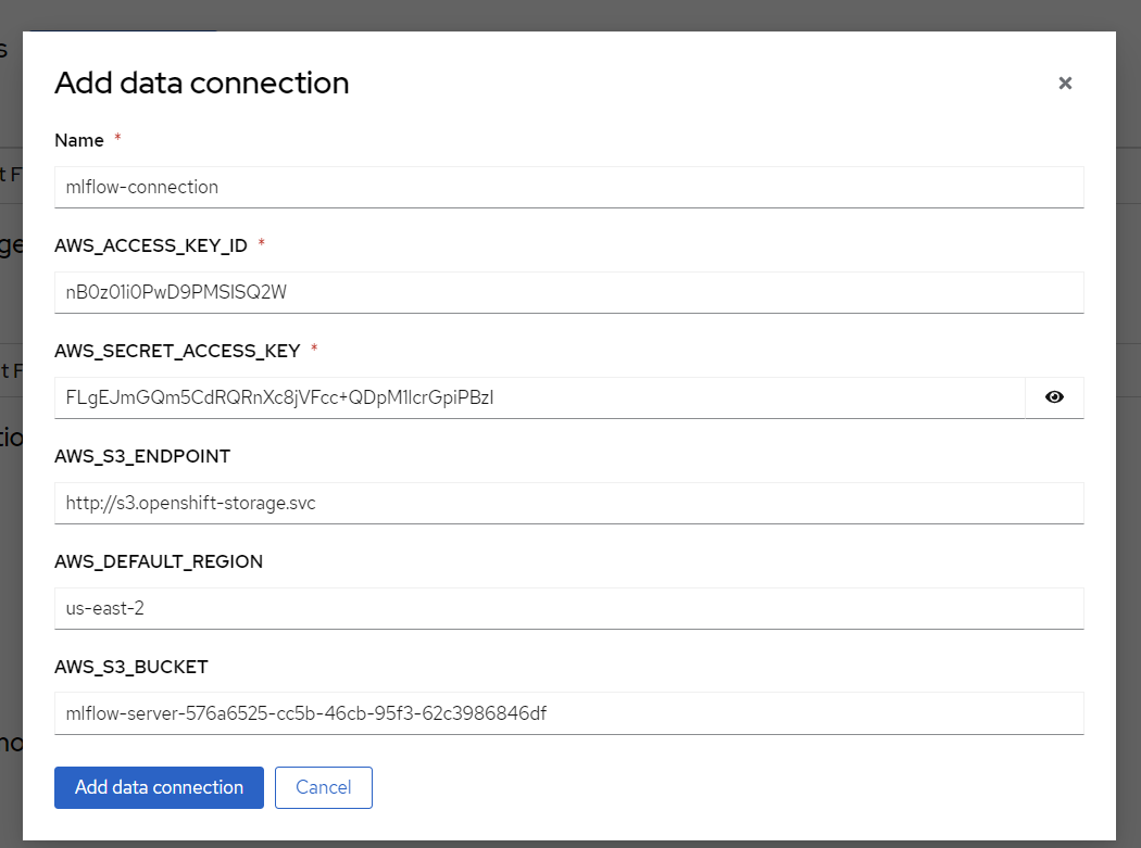
Figure 6. Add data connection details

Next, configure a model server, which will serve our models.

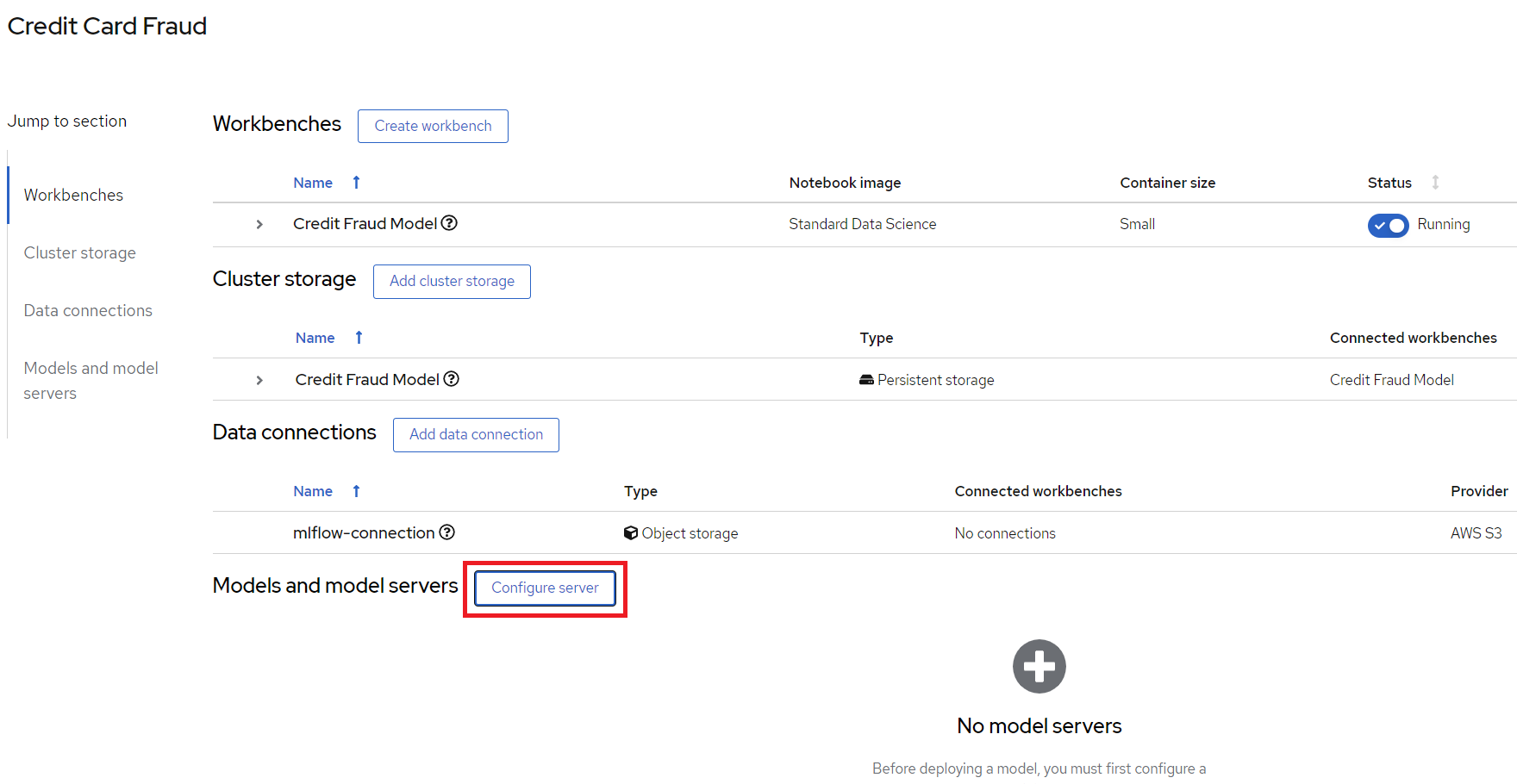
Figure 7. Configure model server

Add Model Server

Model server name = credit card fraud
Serving runtime = OpenVINO Model Server
Model server replicas = 1
Model server size = Small
Check the Make deployed models available through an external route box external access model is required. This is not needed in this dmeo.

Deploy Model

Finally, we will deply the model, to do that, press the "Deploy model" button which is in the same place that "Configure Model" was before. We need to fill out a few settings here:

Name: credit card fraud
Model framework: onnx-1 - Since we saved the model as ONNX in the model training section
Model location:
- Name: mlflow-connection
- *Folder path: This is the full path we can see in the MLFlow interface from the end of the previous section. In my case it’s 1/b86481027f9b4b568c9efa3adc01929f/artifacts/models.Beware that we only need the last part, which looks something like: 1/…./artifacts/models

Note: use models not model. There are 2 folder in MLflow that might cause confusion.

Figure 8. Review MLFlow Model Path

Note the models in highlighted folder.

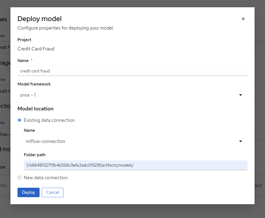
Figure 9. Deploy the Model

Press Deploy and wait for it to complete. A green checkmark will be displayed when done. The status is displayed on the line for model "credit fraud" to the right.

Access the model application

The model application is a visual interface for interacting with the model. You can use it to send data to the model and get a prediction of whether a transaction is fraudulent or not. It is deployed in inferencing-app project. You can access the model application from the images::grid.png short-cut on top right in openshift console: "Inferencing App"

Check the INFERENCE_ENDPOINT env variable value.

Go to https://<your-uri>/ns/inferencing-app/deployments/credit-fraud-detection-demo/environment. Make sure correct INFERENCE_ENDPOINT value is set. In this case it is http://modelmesh-serving.credit-fraud-model:8008/v2/models/credit-card-fraud/infer

You can get this value from

Value: In the RHODS projects interface (from the previous section), copy the "restURL" and add /v2/models/credit-card-fraud/infer to the end if it’s not already there. For example: http://modelmesh-serving.credit-card-fraud:8008/v2/models/credit-card-fraud/infer

Congratulations, you now have an application running your AI model!

Try entering a few values and see if it predicts it as a credit fraud or not. You can select one of the examples at the bottom of the application page.

Next Steps

Help & Feedback Report Bugs