AI Demo | Validated Patterns

AI Demos

First AI demo

In this demo, you will configure a Jupyter notebook server using a specified image within a Data Science project, customizing it to meet your specific requirements.

Procedure

Click the Red Hat OpenShift AI from the nines menu on the OpenShift Console.
Click Log in with OpenShift
Click on the Data Science Projects tab.
Click Create project
1. Enter a name for the project for example my-first-ai-project in the Name field and click Create.
Click on Create a workbench. Now you are ready to move to the next step to define the workbench.
1. Enter a name for the workbench.
2. Select the Notebook image from the image selection dropdown as Standard Data Science.
3. Select the Container size to Small under Deployment size.
4. Scroll down and in the Cluster storage section, create a name for the new persistent storage that will be created.
5. Set the persistent storage size to 10 Gi.
6. Click the Create workbench button at the bottom left of the page.
  After successful implementation, the status of the workbench turns to Running
7. Click the Open↗ button, located beside the status.
8. Authorize the access with the OpenShift cluster by clicking on the Allow selected permissions. After granting permissions with OpenShift, you will be directed to the Jupyter Notebook page.

Accessing the current data science project within Jupyter Notebook

The Jupyter Notebook provides functionality to fetch or clone existing GitHub repositories, similar to any other standard IDE. Therefore, in this section, you will clone an existing simple AI/ML code into the notebook using the following instructions.

From the top, click on the Git clone icon.
In the popup window enter the URL of the GitHub repository in the Git Repository URL field:
```
https://github.com/redhat-developer-demos/openshift-ai.git
```
Click the Clone button.
After fetching the github repository, the project appears in the directory section on the left side of the notebook.
Expand the /openshift-ai/1_First-app/ directory.
Open the openshift-ai-test.ipynb file.
You will be presented with the view of a Jupyter Notebook.

Running code in a Jupyter notebook

In the previous section, you imported and opened the notebook. To run the code within the notebook, click the Run icon located at the top of the interface.

After clicking Run, the notebook automatically moves to the next cell. This is part of the design of Jupyter Notebooks, where scripts or code snippets are divided into multiple cells. Each cell can be run independently, allowing you to test specific sections of code in isolation. This structure greatly aids in both developing complex code incrementally and debugging it more effectively, as you can pinpoint errors and test solutions cell by cell.

After executing a cell, you can immediately see the output just below it. This immediate feedback loop is invaluable for iterative testing and refining of code.

Performing an interactive classification with Jupyter notebook

In this section, you will perform an interactive classification using a Jupyter notebook.

Procedure

Click the Red Hat OpenShift AI from the nines menu on the OpenShift Console.
Click Log in with OpenShift
Click on the Data Science Projects tab.
Click Create project
1. Enter a name for the project for example my-classification-project in the Name field and click Create.
Click on Create a workbench. Now you are ready to move to the next step to define the workbench.
1. Give the workbench a name for example interactive-classification.
2. Select the Notebook image from the image selection dropdown as TensorFlow.
3. Select the Container size to Medium under Deployment size.
4. Scroll down and in the Cluster storage section, create a name for the new persistent storage that will be created.
5. Set the persistent storage size to 20 Gi.
6. Click the Create workbench button at the bottom of the page.
  After successful implementation, the status of the workbench turns to Running
7. Click the Open↗ button, located beside the status.
8. Authorize the access with the OpenShift cluster by clicking on the Allow selected permissions. After granting permissions with OpenShift, you will be directed to the Jupyter Notebook page.

Obtaining and preparing the dataset

Simplify data preparation in AI projects by automating the fetching of datasets using Kaggle’s API following these steps:

Navigate to the Kaggle website and log in with your account credentials.
Click on your profile icon at the top right corner of the page, then select Account from the dropdown menu.
Scroll down to the section labeled API. Here, you’ll find a Create New Token button. Click this button.
A file named kaggle.json will be downloaded to your local machine. This file contains your Kaggle API credentials.
Upload the kaggle.json file to your JupyterLab IDE environment. You can drag and drop the file into the file browser of JupyterLab IDE. This step might visually look different depending on your Operating System and Desktop User interface.
Clone the Interactive Image Classification Project from the GitHub repository using the following instructions:
1. At the top of the JupyterLab interface, click on the Git Clone icon.
2. In the popup window, enter the URL of the GitHub repository in the Git Repository URL field:
  https://github.com/redhat-developer-demos/openshift-ai.git
3. Click the Clone button.
4. After cloning, navigate to the openshift-ai/2_interactive_classification directory within the cloned repository.
Open the Python Notebook in the JupyterLab Interface.
The JupyterLab interface is presented after uploading kaggle.json and cloning the openshift-ai repository shown the file browser on the left with openshift-ai and .kaggle.json.
Open Interactive_Image_Classification_Notebook.ipynb in the openshift-ai directory and run the notebook, the notebook contains all necessary instructions and is self-documented.
Run the cells in the Python Notebook as follows:
1. Start by executing each cell in order by pressing the play button or using the keyboard shortcut "Shift + Enter"
2. Once you run the cell in Step 4, you should see an output as shown in the following screenshot.
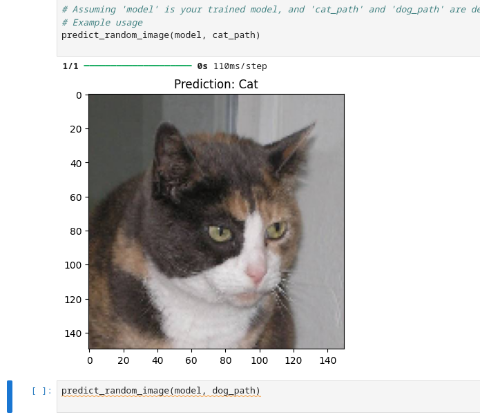
3. Running the cell in Step 5, produces an output of two images, one of a cat and one of a dog, with their respective predictions labeled as "Cat" and "Dog".
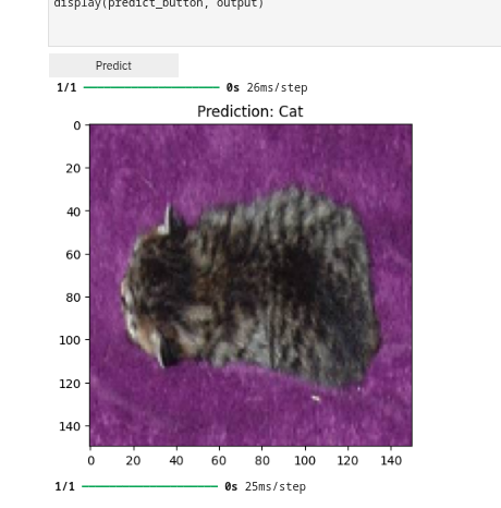
4. Once the code in the cell is executed in Step 6, a predict button appears as shown in screenshot below. The interactive session displays images with their predicted labels in real-time as the user clicks the Predict button. This dynamic interaction helps in understanding how well the model performs across a random set of images and provides insights into potential improvements for model training.

Addressing misclassification in your AI Model

Misclassification in machine learning models can significantly hinder your model’s accuracy and reliability. To combat this, it’s crucial to verify dataset balance, align preprocessing methods, and tweak model parameters. These steps are essential for ensuring that your model not only learns well, but also generalizes well, to new, unseen data.

Adjust the Number of epochs to optimize training speed
Changing the number of epochs can help you find the sweet spot where your model learns enough to perform well without overfitting. This is crucial for building a robust model that performs consistently.
Try different values for steps per epoch.
Modifying steps_per_epoch affects how many batches of samples are used in one epoch. This can influence the granularity of the model updates and can help in dealing with imbalanced datasets or overfitting.

For example make these modifications in your notebook or another Python environment as part of Step 3: Build and Train the Model:

# Adjust the number of epochs and steps per epoch
model.fit(train_generator, steps_per_epoch=100, epochs=10)

Additional resources

Red Hat OpenShift AI learning